Article Text

Abstract
Objective UNAIDS and country analysts use a simple infectious disease model, embedded in the Estimation and Projection Package (EPP), to generate annual updates on the global HIV/AIDS epidemic. Our objective was to develop modifications to the current model that improve fit to recently observed prevalence trends across countries.
Methods Our proposed alternative to the current EPP approach simplifies the model structure and explicitly models changes in average infection risk over time, operationalised using penalised B-splines in a Bayesian framework. We also present an alternative approach to initiating the epidemic that improves standardisation and efficiency, and add an informative prior distribution for changes in infection risk beyond the last data point that enhances the plausibility of short-term extrapolations.
Results The spline-based model produces better fits than the current model to observed prevalence trends in settings that have recently experienced levelling or rising prevalence following a steep decline, such as Uganda and urban Rwanda. The model also predicts a deceleration of the decline in prevalence for countries with recent experience of steady declines, such as Kenya and Zimbabwe. Estimates and projections from our alternative model are comparable to those from the current model where the latter performs well.
Conclusions A more flexible epidemiological model that accommodates changing infection risk over time can provide better estimates and short-term projections of HIV/AIDS incidence, prevalence and mortality than the current EPP model. The alternative model specification can be incorporated easily into existing analytical tools that are used to produce updates on the global HIV/AIDS epidemic.
- HIV
- projection
- dynamic model
- splines
- estimation and projection package
- Mathematical model
- projection
This is an open-access article distributed under the terms of the Creative Commons Attribution Non-commercial License, which permits use, distribution, and reproduction in any medium, provided the original work is properly cited, the use is non commercial and is otherwise in compliance with the license. See: http://creativecommons.org/licenses/by-nc/2.0/ and http://creativecommons.org/licenses/by-nc/2.0/legalcode.
Statistics from Altmetric.com
Introduction
Many countries lack sufficient health information systems to measure the number of individuals living with HIV/AIDS, the rate of new infections, and the need for antiretroviral therapy (ART). To fill this information gap, the UNAIDS Reference Group on Estimates, Modelling and Projections developed, and continues to refine, an epidemiological model for estimation and short-term extrapolation of HIV/AIDS trends from limited surveillance data.1–5 The model (referred to hereafter as the ‘Reference Group model’) is implemented in the freely available Estimation and Projection Package (EPP) and is used by UNAIDS and analysts in countries to generate annual updates on the global HIV/AIDS epidemic.5 6
While the Reference Group model provides a relatively simple tool that produces plausible fits to a wide variety of observed patterns in surveillance data, a number of specific patterns have been challenging to reproduce. Examples include countries in which observed prevalence has declined sharply and then levelled off, and countries in which prevalence has been steadily increasing or decreasing.5 Other concerns have been noted regarding short-term projections of prevalence approaching zero in several settings, which are regarded as epidemiologically implausible.5 These limitations of the model stem in part from its approach to approximating changes in infection risk over time,7 which may result from the spread of an epidemic in a population with heterogeneous risk behaviour, or from changes in individuals' sexual behaviour.8 9
The rapid rise in prevalence in the early years of many African epidemics is consistent with a high initial force of infection on average, as the epidemic begins to spread among a population with relatively high-risk behaviours. However, if this high average infection rate were to persist as HIV expanded into the general population, prevalence would reach unrealistically high levels. To address this dynamic, the Reference Group model partitions the uninfected population into two risk groups, ‘susceptible, not at-risk’ and ‘susceptible, at-risk’. The fraction of the population initially in the ‘susceptible, at-risk’ compartment constrains the peak prevalence level. The rate at which prevalence declines after its peak is determined by the balance between new infections and mortality, and can be modulated in the Reference Group model to a limited degree by adjusting the fraction of new adults entering the ‘susceptible, at-risk’ population.2 Overall, the Reference Group model specification is well suited to characterising various patterns of prevalence during the early phase of an epidemic and in the time shortly after a peak, but the model is less flexible in accommodating different types of trajectories as epidemics move further in time beyond peak prevalence.
Modifications to the Reference Group model that enable better fits to prevalence data should meet several criteria. First, a modified model should maintain the explicit connection in the current model between prevalence of infected people and the risk of infection among uninfected people. Models that fit curves directly to prevalence data without explicitly modelling the underlying infection dynamics might, for example, produce a prevalence curve that would imply a negative incidence rate. Another argument for maintaining an explicit epidemiological model (as opposed to a curve-fitting approach) is to accommodate estimation of incidence and mortality patterns, scenario analyses and future predictions. Second, parsimony is important as many settings do not have the data required to parameterise more complex models, such as those that incorporate age structure, detailed patterns of sexual behaviour, or expanded risk group structure.10–12 Simpler models also require less computational power, which is an important consideration for end-users of EPP. Finally, a modified model for EPP should be flexible enough to fit a variety of epidemic trajectories around the world.
Previously, we suggested a relatively parsimonious modification to the Reference Group model that would eliminate the current partitioning of the susceptible population into ‘at-risk’ and ‘not-at-risk’ segments, but would allow the average infection rate to change over time.7 From an epidemiological standpoint, such an approach should respect the weak constraint that changes in the infection rate should be relatively smooth over the course of the epidemic. In this paper, we present a specific operationalisation of this alternative approach using penalised B-splines to model the annual infection rate parameter as a function of time. Our proposed model adds two further modifications to the current model, which provide (1) a more standardised and efficient way to model the initial phase of an epidemic, and (2) improved plausibility of extrapolations beyond the last observed data point by incorporating an informative prior distribution for short-term projections of infection risks.
Methods
Data sources
For many generalised epidemics, such as those in sub-Saharan Africa, the primary source of time series data on HIV prevalence is a system of sentinel surveillance sites that undertake anonymous HIV-prevalence testing of blood samples from pregnant women attending antenatal clinics (ANC).13 Use of ANC data has been justified based on the argument that prevalence among pregnant women serves as a reasonable proxy for prevalence in the general adult population, although some concerns have been noted about the representativeness of the sample and the possible effects of changing rates of contraceptive use over time.14 15 More recently, results from national population-based surveys have indicated that ANC data tend to overestimate prevalence in the general population.16 Since these surveys are only available for 1 or 2 years in most countries, the Reference Group model uses ANC data to inform the shape of prevalence over time and calibrates this curve to match the level of the national population-based survey estimates when available.5 As we are primarily concerned in the present study with characterising the shape of prevalence curves generated under alternative models, we omit this calibration step here in order to facilitate visual inspection of model output in relation to empirical ANC data. Our approach, however, generalises easily to a more detailed overall modelling approach that includes calibration to estimates from national surveys.
We fit the model separately to a total of 18 populations, distinguishing urban from rural regions in nine countries: Angola, Burundi, Ethiopia, Gabon, Kenya, Lesotho, Rwanda, Uganda and Zimbabwe. Rwanda and Uganda offer two important examples in which the Reference Group model fails to capture recent trends in prevalence.
Proposed model
Our proposed alternative to the current EPP model explicitly represents changes in infection risks over time to better approximate patterns of HIV spread in generalised epidemics. We simplify the population structure of the Reference Group model by collapsing the ‘susceptible, at-risk’ and ‘susceptible, not at-risk’ compartments into one uninfected (and at-risk) sub-population. In line with the modified structure, we remove two corresponding parameters from the Reference Group model — f0, which governs the initial split between at-risk and not-at-risk entrants, and φ, which modulates this split in mature epidemics. In assessing the performance of the spline-based approach, we limit our analysis to scenarios that do not include ART, although we note again that our approach generalises easily to a more detailed specification including ART.
The model can be described by three differential equations, following the general notation for the Reference Group model used in EPP 200917:
The key difference in the parameterisation of this model compared with that in the current Reference Group model is the use of a time-varying function for infection risks, r(t), modelled using splines, rather than assuming constant r. A number of other key elements of the model are consistent with the current Reference Group formulation. The model distinguishes early-stage from late-stage infection (eg, those having CD4 counts above or below 200 cells/μl) in order to accommodate the modelling of treatment eligibility. Y represents the number of HIV-positive individuals at the earlier stage, U is the number of HIV-positive individuals at the later stage, and Z is the number of uninfected individuals (Y+U+Z=N). E(t) is the number of new adults entering the population at time t and is a function of HIV prevalence 15 years earlier, which accounts for differential fertility and child survival by maternal HIV status. The functions g1(x) and g2(x) determine HIV disease progression, from the early to the more advanced stage, and from the advanced stage to AIDS-related death, respectively. Both functions are parameterised as Weibull densities, with shape and location parameters α=1.69 and β=10.40 for g1(x) and α=1.00 and β=2.52 for g2(x), yielding median residence times of 8.4 and 1.8 years, respectively.
We make another important modification to the Reference Group model by changing the way in which the model captures the initial phase of an epidemic. Fitting the Reference Group model currently requires estimation of the year (t0) in which a fixed seed value of Yt0=0.0025 initiates the epidemic. In our proposed specification, an epidemic is initiated in 1975 with a small pulse of infected individuals Y0, which is a parameter to be estimated with a broad prior uniform distribution spanning the range 10−13 to 0.0025. Given the large uncertainty about when HIV first appeared in human populations,18 and the inevitable artifice of simulating the introduction and initial spread of HIV as a discrete event, this new approach avoids having to estimate the ‘start year' of the epidemic, while acknowledging substantial uncertainty about the early dissemination of HIV through the population. It also ensures a constant number and position of splines for the r function and improves efficiency, as the fitting algorithm no longer needs to be re-run for each potential value of t0.
There are several possible choices of spline functions for modelling infection risks over time, r(t).19 20 We propose to use third degree B-splines with a difference penalty to enforce smoothness (also referred to as ‘P-splines’).21 B-splines are easy to generate (the basis functions consist of polynomial pieces) and have stable boundaries. With this formulation, a relatively large number of basis functions can be set at equal intervals, and a difference penalty on the coefficients of adjacent basis functions determines the amount of smoothing.21 Here we use a second-degree difference penalty, which enforces smoothness in the second derivative of the spline function (ie, smooth changes in the slope of r over time in the epidemic model). Figure 1 shows an example of how one trajectory for r(t) (thick solid line) is generated from seven B-spline basis functions (dotted lines), as used in our analysis. The function r(t) is constructed as a linear combination of the basis functions, with the spline coefficients (denoted β1 through β7) serving as weights.
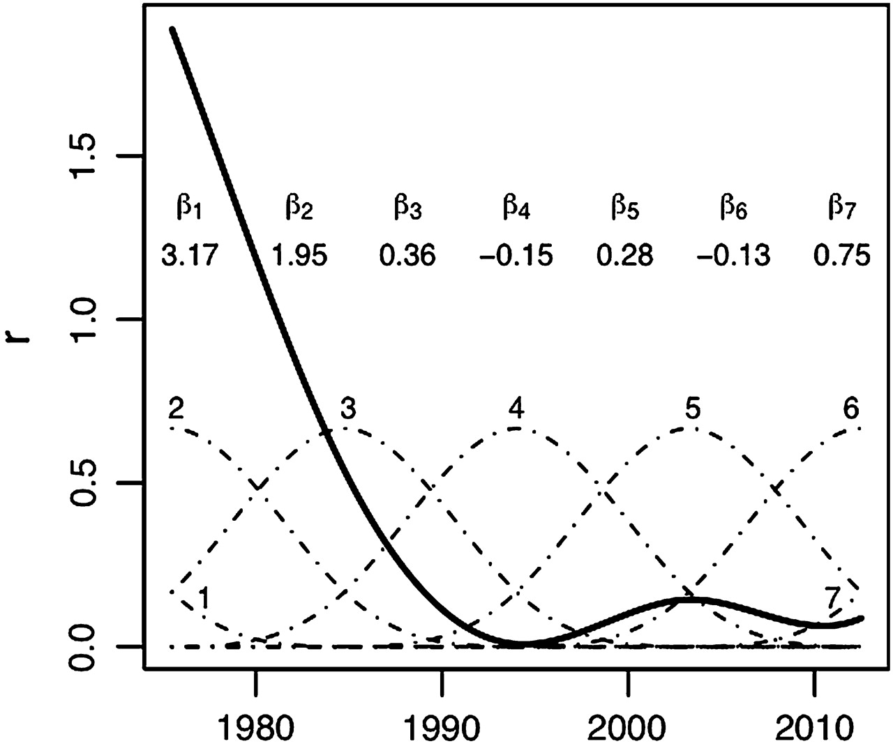
Example of a spline-based curve for infection risks over time (solid line) using third degree B-splines comprised of seven evenly-spaced basis functions (dashed curves labelled 1 through 7). The spline curve is a linear combination of the basis functions and their coefficients (labelled β1 through β7).
In line with the current strategy for estimating model parameters and characterising uncertainty, we adopt a Bayesian approach to fitting the model to surveillance data,22 specifically using a Bayesian analogue to B-splines with difference penalties.23 For the second-degree difference penalty used here, the coefficient for basis function i is expected to follow the trend of the previous two coefficients, and its prior can be expressed as: βi=βi -1+(βi -1–βi -2)+ui. The priors for β1 and β2 are assumed to be proportional to a constant. Note that if all of the β coefficients are equal, the resulting ‘curve’ will be a horizontal line. On the other hand, if a spline coefficient differs greatly from its neighbouring coefficients, we expect the curve to change in value rather quickly over the range of that basis function. By letting ui ∼ normal(0,τ2), the amount of smoothness is determined by the variance parameter τ2, as smaller values for τ2 will produce smaller values for ui, which in turn imply a smoother function. The parameter τ2 is estimated during model fitting, and we use the common uninformative prior τ2 ∼ inverse-gamma(0.001,0.001).24 In preliminary analyses we tested between four and 10 evenly-spaced basis functions and found that seven basis functions were sufficient to obtain adequate flexibility for r(t) to match a wide variety of different empirical prevalence trends. When fitting the model, we add a further constraint that r must always be positive.
Short-term projections
While the primary objective of the model described here is to estimate past epidemic trends for reporting on the current status of HIV/AIDS epidemics, one of the required functions of the model is to make short-term projections beyond the last observed data point in settings that lack data for the most recent reporting year(s). There are a range of methodological challenges in extrapolating time series beyond the last observed data point, including both general challenges and certain challenges specific to spline models.25 26 In order to address the challenge of extrapolation, we incorporate a prior probability distribution for future values of r derived from observed prevalence levels in the most recent years of data. The specification of the prior draws on the mathematical theory of infectious disease dynamics.27 Briefly, if we let I be the proportion infected and S be the proportion uninfected, with infection rate r and mortality rate μ, the change in the infected population is given by dI/dt=rIS–μI. At later stages in an epidemic, we expect prevalence to approach equilibrium, all else being equal. Under this formulation, dI/dt=0 when r=μ/S, which we approximate as r≈1/(1– prevalence)×1/duration. (This is an approximation given a non-constant mortality rate for HIV/AIDS.) With the mortality assumptions in EPP 2009, mean duration with HIV/AIDS is approximately 11.5 years. We implement this prior for r(t) by assuming that future values of r are normally distributed, with mean r(t)=1/(1–Y(t*)/N(t*))×1/11.5, where Y(t*)/N(t*) is modelled prevalence in the last year of data. Variance of the distribution is set equal to the mean of the squared deviations between r(t) and 1/(1–Y(t)/N(t))×1/11.5 for the last 10 data-supported years of the projection. The prior is included in the model fitting process and serves to guide the spline curve (which is generated as a continuous function for the entire estimation and projection period) beyond the last observed data point.
We note that this prior is intended only to ensure that most curves for r reside within a reasonable range for later-stage, fully generalised epidemics, and not necessarily to capture long-term dynamics in future predictions. By ‘reasonable range’, we suggest, for example, that an annual value of r=1, which implies an average of more than 11 secondary infections over the lifetime of an infected person, would be unreasonably high for a late-stage epidemic as illustrated by Uganda in 2010, given that the average lifetime number of sexual partners has been estimated at around 2–3 for women and 10 for men across several African studies,28 and that most partnerships do not result in infection (the average probability of transmission in a single sexual act has been estimated to be as low as 1 per 1000).29 A recent modelling study based on long-term follow-up of a cohort in Rakai, Uganda estimated that approximately two new infections would be generated by each infected individual based on random mixing in sexual partnerships,30 which underscores that values for r should be much less than 1 and within the range implied by the prior used here for future values of r.
Model fitting
Following the work of Bao and Raftery, we use incremental mixture importance sampling (IMIS) for model fitting, which is a Bayesian algorithm for simulating posterior distributions.31 We employ the same likelihood as that used currently in EPP, which assumes that prevalence is normally distributed on the probit scale, with random effects for ANC sites.32 The spline-based model was programmed in the software package R, with some functions written in C to increase computational speed, and the model differential equations were approximated as difference equations in quarter-year increments. For comparison with the existing Reference Group model, results were obtained by running the uncertainty analysis option in EPP 2009. For the spline-based model, we added the additional constraints that r <20 and prevalence <95% to increase the efficiency of the IMIS algorithm. These constraints allowed us to avoid calculating the likelihood for proposed parameter sets that led to epidemiologically implausible epidemic trajectories. The choice of r <20 was a very weak constraint; we did not observe values of 10 or greater in the posterior distributions of r for any country. We started the IMIS algorithm with 900 000 initial draws, with 900 draws for each importance sampling iteration.
Model evaluation
We compared the alternative models in terms of their observed fit to surveillance data from all sites. The performance of the models was also evaluated based on more formal criteria. To compare the relative fit of the spline-based and Reference Group models to ANC data, we computed Bayes factors33 along with density plots of the marginal likelihoods for both models. We further evaluated the spline-based model with posterior predictive checks of in-sample fit by comparing posterior predicted prevalence to observed prevalence for each site-year observation. We performed these posterior predictive checks after constructing case-deleted posteriors for each ANC site's random effect via sample reweighting,34 and we obtained predicted random effects for ANC prevalence via rejection sampling.32 To assess the model's performance in out-of-sample projection, we truncated the last 3 years of data, re-fit the model and determined if the 95% credible intervals for prevalence covered the median projection from the model fit to the full ANC time series. We tested the robustness of the IMIS algorithm by re-running our standard projections with a different random seed and comparing the posteriors for r, incidence and prevalence. We also investigated the sensitivity of the results to the prior on τ2, and we visually compared posterior distributions of each model parameter to the distribution of initial draws for the IMIS algorithm.
Results
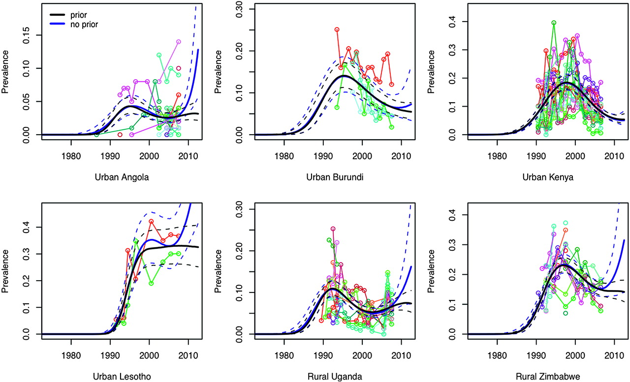
As shown by the illustrative examples in figure 2, the spline-based model appears to out-perform the Reference Group model in capturing trends in prevalence in countries that have recently experienced a levelling off or rise in prevalence following a steep decline (see urban and rural Uganda, urban Rwanda and rural Burundi). The spline-based model also predicts a deceleration of the decline in prevalence for countries that have recently experienced steady declines, such as Kenya and Zimbabwe. Bayes factors indicate that the spline-based model produces a better fit to ANC data than the original Reference Group model for all 18 settings examined (all values for 2 log(BF)>7), including those settings in which the Reference Group model produces a reasonable visual fit to the data.

Median prevalence with 95% credible intervals (in black) for the spline-based model for r, with the best fit from the EPP 2009 Reference Group model added for comparison (in blue) for nine selected settings. Observed prevalence data for antenatal clinic sites to which the models are fit are plotted in various colours.
Posterior predictive checks suggest that the spline-based model predicts the observed data well across and within sites. Figure 3 shows examples from Uganda. Predicted prevalence across all ANCs was highly consistent with observed prevalence overall, and site-level prediction intervals for prevalence typically contained the observed values. Exceptions included some instances in which the model over-predicted low-prevalence values; however, we note that in these instances comparable or greater errors were observed in the Reference Group model. A small number of very high prevalence values were under-predicted by both models.

Posterior predicted prevalence versus observed prevalence across all antenatal clinic sites for urban and rural Uganda, along with posterior predicted site-level prevalence for four selected antenatal clinics (red indicates observed site prevalence, black indicates median and 95% prediction intervals for predicted site prevalence).
The IMIS algorithm was largely insensitive to initial conditions. In comparing posterior projections from the algorithm started with two different random seeds, estimated values for r during the early phase of the epidemic varied between simulations for some countries. However, initial patterns of incidence (and prevalence), which are determined by the combination of r and the initial pulse of infection Y0, were much more similar, and patterns of r converged by the time prevalence peaked. (The IMIS algorithm clearly outperformed a Markov Chain Monte Carlo sampler with respect to convergence.) Trajectories for r, incidence, and prevalence from a model which assumed τ2 ∼ uniform(0,30) were similar to the τ2 ∼ inverse-gamma(0.001,0.001) prior model, with some differences in early-stage estimates for urban Burundi and rural Rwanda.
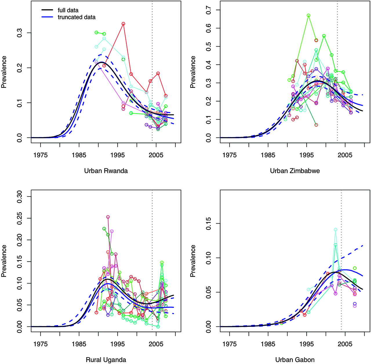
The model we propose here incorporates an informative Bayesian prior probability distribution for projections of r beyond the last observed data point. We evaluated this modelling choice in two ways. First, we examined whether including the prior alters in-sample estimates compared with a model without a prior. Across the 18 settings included in our analysis, the prior had little discernible impact on in-sample fit, particularly after the peak in prevalence (figure 4). Second, we tested the model's ability to extrapolate beyond the last observed data point (ie, to predict out-of-sample) by deleting the last 3 years of observed data for each setting, and then refitting the model to determine if the uncertainty bounds for the out-of-sample predictions contained the original data-supported median predictions. Performance of out-of-sample predictions was strongest where several years of observed data were available after the epidemic peak (figure 5). Out-of-sample prediction errors were largest in settings with relatively sparse data, or settings in which the last data points occurred around the time that prevalence was peaking (as in Gabon). The model also failed to predict the exceptional, sudden reversal observed in rural Uganda. In this latter case, given a point of inflection coinciding almost precisely with the truncation of the data, we expect that out-of-sample predictions from any model would likely suffer from similar imperfections. For 3-year out-of-sample predictions, the median full data prediction fell within the 95% credible intervals for 12 out of 18 settings.
Median prevalence with 95% credible intervals for the spline-based model with (in black) and without (in blue) a prior for the future behaviour of r for six selected settings. Observed prevalence data for antenatal clinic sites to which the models are fit are plotted in various colours.

Median prevalence with 95% credible intervals for out-of-sample prevalence predictions for the spline-based model (in blue), with median fit for the full-sample results added for comparison (in black), for four selected settings. Data for the last 3 years of observation were excluded for generating out-of-sample predictions (denoted by the vertical dashed line).
As rising coverage of ART makes interpretation of trends in prevalence increasingly complicated, there has been a corresponding shift in emphasis towards measurement and modelling of incidence. This shift is reflected in the most recent changes to the suite of tools used by UNAIDS and country analysts in their routine updates on the status of HIV/AIDS epidemics.17 In light of this shift in emphasis, it is critically important that evaluation of alternative models includes assessment of estimated trends in r, incidence and mortality as well as trends in prevalence. As shown in figure 6 for urban Uganda and urban Rwanda, incidence may be increasing even in the presence of declining prevalence. The general pattern of r shown in figure 6, with r starting at a high value and then falling to lower levels, is common across the 18 settings included in this study and is consistent with our understanding of how the force of infection should change as an epidemic becomes generalised. The pattern for r over the last 5 years of the projection was more variable across countries, which underscores recent concerns about potential reversals in progress on preventing risky behaviours in some settings.

Plots of r, incidence and mortality for urban Uganda and urban Rwanda from the spline-based model. Unique curves from the posterior are plotted in grey, along with the median and 95% credible intervals.
Discussion
Our investigation into relaxing the UNAIDS Reference Group model's assumption of a constant infection rate parameter over time suggests that it is feasible to obtain better fits to recent prevalence data, as evidenced by the flexible model's ability to capture recent trends in Uganda and Rwanda. The model also shows promise in avoiding projected prevalence declining towards zero for epidemics like that in Kenya. Using splines to model r as a function of time directly addresses changing infection risk while respecting basic epidemiological constraints and maintaining smooth patterns of r, incidence, mortality and prevalence.
Several limitations in the proposed model should be noted. The spline-based approach in the formulation presented here yielded divergent out-of-sample predictions in some countries. It is worth noting, however, that the out-of-sample prediction errors typically occurred in settings where predictions were made in close proximity to an epidemic peak. For the intended use of this model, most generalised epidemics have advanced sufficiently beyond the peak that the required out-of-sample predictions should be less vulnerable to error. The choice of prior for r to enable short-term future predictions also has limitations. First, it assumes that an epidemic is trending towards equilibrium. Second, it assumes a constant mortality rate, which is an approximation of a more complicated pattern of survivorship, and the inclusion of disease-induced mortality can alter the equilibrium dynamics of epidemic models.35 Further examination of alternative specifications for the Bayesian prior on r might reveal better options.
An important limitation in both the flexible model and the Reference Group model is that they focus on average rates of infection and mortality across the entire adult population, thus summarising the dynamics of HIV spread through a heterogeneous population with a few equations instead of explicitly modelling the distribution of risk behaviours across individuals and accounting for the age structure of the population.10–12 Our proposed approach has some advantages in this regard compared with the current model. Allowing r to change over time approximates the dynamics associated with HIV spreading into the general population as an epidemic progresses, while still maintaining the parsimonious framework of the Reference Group model. The spline-based approach also generates smooth patterns of incidence and mortality, unlike a pragmatic approach to increasing the flexibility of the Reference Group model that allows for a shift in the proportion of new adults recruited to the at-risk population.17
In comparison to the Reference Group model, the spline-based approach imposes somewhat greater computational demands. With seven spline basis functions there are a total of nine parameters to estimate, compared with four in the Reference Group model. On average the IMIS algorithm needed to calculate twice as many likelihoods when fitting the spline-based model as when fitting the Reference Group model. The relatively common shape of r over time across countries suggests that computation could be made more efficient by centering the initial draws for the IMIS algorithm on more plausible values. The similarity in patterns of infection risk across countries also suggests that hierarchical modelling of multiple epidemics could improve estimates for countries with sparse data and may be a fruitful area for future research. The incorporation of age structure into a flexible model for r is another potential area for further study.
By obtaining better projections of HIV/AIDS epidemic dynamics, a modification to the Reference Group model that allows r to vary over time has the potential to improve the accuracy of estimates that are used by decision makers to track the state of the epidemic and to plan future health resource needs. Future research on flexible modifications to the Reference Group model should include a careful consideration of ART provision, which not only affects survivorship but also transmission rates for those receiving treatment. Both effects can be accommodated with the model proposed here, and they will be important for obtaining accurate estimates of incidence from prevalence in the coming years, as increases in prevalence may be due to decreases in mortality as well as new infections. Finally, the performance of a flexible function for r should be explored in the context of countries with concentrated epidemics, which may require stronger modelling assumptions to overcome the difficulties in fitting curves to distinct sub-epidemics with little surveillance data.
Acknowledgments
The authors gratefully acknowledge helpful inputs from Leontine Alkema, Le Bao, Tim Brown, Peter Ghys, Chris Paciorek, Adrian Raftery and Karen Stanecki.
References
Footnotes
Funding This study was supported in part by funding from the UNAIDS Reference Group on Estimates, Modelling and Projections, and by a T32 training grant from the National Institute of Allergy and Infectious Diseases (AI 007433).
Competing interests None.
Provenance and peer review Not commissioned; externally peer reviewed.