Article Text

Abstract
Objective United Nations Programme on HIV/AIDS reports regularly on estimated levels and trends in HIV/AIDS epidemics, which are evaluated using an epidemiological model within the Estimation and Projection Package (EPP). The relatively simple four-parameter model of HIV incidence used in EPP through the previous round of estimates has encountered challenges when attempting to fit certain data series on prevalence over time, particularly in settings with long running epidemics where prevalence has increased recently. To address this, the most recent version of the modelling package (EPP 2011) includes a more flexible epidemiological model that allows HIV infection risk to vary over time. This paper describes the technical details of this flexible approach to modelling HIV transmission dynamics within EPP 2011.
Methodology For the flexible modelling approach, the force of infection parameter, r, is allowed to vary over time through a random walk formulation, and an informative prior distribution is used to improve short-term projections beyond the last year of data. Model parameters are estimated using a Bayesian estimation approach in which models are fit to HIV seroprevalence data from surveillance sites.
Results This flexible model can yield better estimates of HIV prevalence over time in situations where the classic EPP model has difficulties, such as in Uganda, where prevalence is no longer falling. Based on formal out-of-sample projection tests, the flexible modelling approach also improves predictions and CIs for extrapolations beyond the last observed data point.
Conclusions We recommend use of a flexible modelling approach where data are sufficient (eg, where at least 5 years of observations are available), and particularly where an epidemic is beyond its peak.
- AIDS
- Statistics
- Epidemiology (General)
This is an open-access article distributed under the terms of the Creative Commons Attribution Non-commercial License, which permits use, distribution, and reproduction in any medium, provided the original work is properly cited, the use is non commercial and is otherwise in compliance with the license. See: http://creativecommons.org/licenses/by-nc/3.0/ and http://creativecommons.org/licenses/by-nc/3.0/legalcode
Statistics from Altmetric.com
Introduction
Every 2 years, the Joint United Nations Programme on HIV/AIDS (UNAIDS) produces estimates and projections of HIV/AIDS prevalence, incidence and mortality by country.1 The technical basis for this effort has been guided by recommendations from the UNAIDS Reference Group on Estimates, Modelling and Projections, and a suite of analytic tools has been developed for this purpose, including the UNAIDS Estimation and Projection Package (EPP)2–7 and Spectrum.8–12 EPP fits an epidemiological model to prevalence data obtained from sentinel surveillance systems and national population-based HIV seroprevalence surveys, and Spectrum translates estimates of HIV incidence into a range of corresponding population health consequences, including AIDS mortality. For the most recent round of estimates, EPP and Spectrum have been integrated into a single software package.
The first widely available version of EPP in 2003 incorporated a simple four-parameter model patterned after the epidemiology of HIV in closed populations.2 This model provided a good fit to most generalised epidemics, but in concentrated epidemics sometimes failed to produce flat enough curves for populations with high levels of turnover, for example, injecting drug users (IDU). This problem was addressed in EPP 2005, which allowed for movement between populations.4 However, in the 2007 round of projections limitations in the simple four-parameter model became apparent in a few countries. In two countries incidence in the fitted models fell unrealistically to zero in the near future. In two other countries the model was unable to replicate plateauing prevalence trends at levels well below the peak prevalence or to reproduce epidemics where prevalence was again rising after a steep initial decline. The simple four-parameter model was not sufficiently flexible to allow for complex trends after the epidemic peak. To address this issue, EPP 2009 included an optional modification to accommodate increases in prevalence following a period of decline by replenishing the susceptible pool,7 but this modification was not sufficient and proved to have limited utility.
To deal with these more variable epidemiological patterns appearing in some long running epidemics, an alternative approach was suggested in which the model allows the average infection rate in a population to vary over time. Two specific formulations of this approach were proposed: one parameterised a time series of infection risks using penalised B-splines,13 and another assumed that infection risks follow a Gaussian random walk with mean zero.14 These flexible models appeared to provide better fits to recent prevalence trends in several cases.
Here we describe the flexible epidemiological model implemented in the UNAIDS EPP 2011 (hereafter EPP 2011), which was developed from the previously proposed spline and random walk models. In the Methods section we review the general modelling approach in EPP, contrast the ‘classic’ and flexible epidemiological models, and summarise the Bayesian estimation method used for model fitting. In the Results section, we present illustrative prevalence and incidence trajectories for 10 countries with generalised epidemics and 6 countries with concentrated epidemics, as well as a summary of formal out-of-sample projection tests. In the Discussion section, we offer some conclusions and highlight model settings that the end-user of EPP 2011 can alter if desired.
Methods
Overview of estimation procedure
Due to the paucity of reliable information on HIV incidence in developing countries, sentinel surveillance systems for HIV were designed to provide information on prevalence trends to policy makers and programme planners. The main data source used in EPP is surveillance data from various sites and years showing HIV prevalence among antenatal clinic (ANC) patients and key populations with elevated HIV risk, for example, men who have sex with men (MSM) or female commercial sex workers (FSW). The ANC data are primarily used to estimate prevalence in the general population while the other data are used to estimate prevalence among higher-risk populations. HIV prevalence among ANC patients has been shown to be somewhat higher than that in the general population.15 In an attempt to obtain more representative estimates of HIV prevalence, since 2001, 32 countries in sub-Saharan Africa have conducted national population-based household surveys, including Demographic and Health Surveys and AIDS Indicator Surveys. These national population-based HIV surveys are used in generalised epidemics to calibrate overall population prevalence levels estimated from ANC surveillance data.16 ,17
The UNAIDS EPP is based on a simple susceptible-infected-recovered epidemiological model, formulated as a set of differential equations, and described in the next section. To obtain probabilistic estimates and projections, a Bayesian approach is used to integrate ANC surveillance data with the modelled estimates of HIV/AIDS prevalence over time.7 ,16 Formally, the epidemiological model provides a deterministic mapping from a vector of input parameters, θ, to a vector of model outputs on prevalence by year, ρ. A prior distribution is specified for the model input parameters, and observed surveillance data give the likelihood L(ρ) for the model output, using a hierarchical random effects formulation. A prior on the model output ρ can also be specified, using the Bayesian melding approach.18 ,19 The chief endpoints of interest in this estimation approach are the posterior distributions for prevalence and incidence over time, the latter taken as an input for further analysis (of endpoints such as AIDS mortality) in Spectrum.
The posterior distribution in EPP is estimated using the incremental mixture importance sampling algorithm.20 The basic idea is to approximate the posterior distribution gradually by a mixture of Gaussian components and the prior distribution, and it works as follows: (1) In an initial stage, a large number of samples are drawn from the prior distribution for the input parameter vector. For each sampled parameter vector, the model is run, and the outputs used to compute the likelihood. Importance weights are proportional to the likelihood, with high importance weights indicating areas where the target density is under-represented by the importance sampling distribution. (2) In an importance sampling stage, undertaken over k iterations, further inputs are drawn from a multivariate Gaussian distribution centred at the current maximum-weight input. Therefore, the new inputs fill in the under-represented parts of parameter space iteratively. (3) In a resampling stage, once a specified stopping criterion is satisfied, a number of resampled input parameter vectors are drawn with replacement, based on their importance weights. We chose 3000 resamples for the EPP 2011 implementation. For each input parameter vector in the resample, quantities of interest computed by running these parameters through the model (eg, HIV prevalence and incidence over time) are realisations from their posterior distributions. The algorithm ends when the expected fraction of unique points in the resample is at least 1−1/e=0.632. This is the expected fraction when the importance sampling weights are all equal, which is the case when the importance sampling function is the same as the posterior distribution.
Epidemiological model in EPP 2011: ‘classic’ formulation
The basis for modelling HIV incidence in the ‘classic’ formulation of the epidemiological model in EPP has been described in detail elsewhere.3 ,5 ,7 Briefly, the population 15 years and older is divided into those not at risk; those at risk, but not yet infected; and those at risk and living with HIV. Modelling of the transmission of HIV infection is governed by four parameters: r, the rate of infection, assumed constant, t0, the start year of the epidemic, f0, the initial fraction of the adult population at risk of infection, and φ, a parameter modulating the split between at-risk and not-at-risk populations in mature epidemics. In the epidemic start year, 0.025% of the at-risk but not yet infected group moves to the infected group to initialise the epidemic. The number of new entrants at time t depends on the population size 15 years earlier, the birth rate and the survival probability from birth to age 15.
As described elsewhere in this supplement,21 EPP 2011 has been expanded to track the infected population's progression across CD4 cell count levels. CD4 counts are also used to improve the realism of the effects of antiretroviral therapy. The new implementation also includes more detailed population demographics, for example, ageing out at age 50 and migration.
Epidemiological model in EPP 2011: flexible formulation
In EPP 2011, the option to run the classic model is retained, but a new flexible specification for modelling transmission is added as an option. The flexible model diverges from the classic model in three key ways. The at-risk and not-at-risk groups are combined, the infection rate r is allowed to vary over time in a flexible way and therefore specified as r(t), and an equilibrium constraint is imposed on projections beyond the last year of data, to avoid explosive behaviour. These changes are described in the following subsections.
Combining the at-risk and not-at-risk groups
The flexible model drops the distinction between individuals at risk and not at risk of infection, treating all HIV negative persons as being at risk.13 ,14 It divides the 15–49 year-old population at time t into two general groups: Z(t) is the number of uninfected individuals and Y(t) is the number of infected individuals. For parsimony in presentation, we describe here a simplified version of the model without the details on CD4 progression that are included in the actual EPP 2011 model. The simplified dynamics are as follows: 1where N(t)=Z(t)+Y(t) is the total population size, E(t) is the number of new adults entering the population, r(t) is the average infection risk, −a50(t) is the rate at which adults exit the model after attaining age 50, and M(t) is the rate of net migration into the population.
Flexible specification for the infection rate, r(t)
The infection rate, r(t), is the expected number of persons infected by one HIV positive person in year t in a wholly susceptible population. In the flexible model formulation, r(t) is modelled as a random walk on the log scale; specifically the first difference is modelled as a series of independent and identically distributed normal random variables, each with mean zero and SD σ:14 2
2
There are often no data in the early period of the epidemic. Let t0 be the start year of the epidemic and t1 be the first year of the observed data. We use the fact that, from (2), log r(t1)−log r(t1)∼N(0, (t1−t0)σ2), and divide the changes from r(t0) to r(t1) equally between each of the years of the ‘pre-data’ period.
Previous versions of EPP estimated the year t0 in which 0.025% of the uninfected population is moved into the infected category in order to initiate the epidemic. In the flexible model, we fix t0 at 1975 and estimate the initial seed y(t0) and initial infection rate r(t0) as parameters, to improve the efficiency of the programme.13
We carry out Bayesian estimation with the following prior distributions: 3
3
The lower bound of r(t0) for generalised epidemics is set at 1/11.5 because the epidemic would not spread if r(t0) were smaller than 1/11.5, since 11.5 is the expected length of the infectious period. The alternative lower bound, 1/11.5+1/d, is recommended for concentrated epidemics, where d is the mean duration that people stay in the at-risk category. We chose ν=10 and λ=0.09 to accommodate the observed changes in all the countries we have considered.
The random walk model for r(t) was realistic for most countries, but gave a posterior distribution of the incidence pattern over time that had two unrealistic peaks in the mid-1990s in Kenya. We put constraints on incidence rates directly, which follows the idea of Bayesian melding.17 Specifically, we set an upper bound, 0.2, on the average of the absolute values of the 2nd derivatives of incidence rates to eliminate the bumpy incidence curves.
To improve sampling efficiency, we integrate out σ2 analytically, so that it is not included in the sampling algorithm. Additionally, we include an optimisation stage after the initial sampling stage in the incremental mixture importance sampling procedure to reduce the time required for convergence. Specifically, we set the maximum weight input from the initial stage as the starting point, use the Nelder-Mead and Broyden-Fletcher-Goldfarb-Shanno (BFGS) methods to obtain a local maximum of the posterior density of the input parameter vector, θopt,22–24 and store the estimated inverse of the Hessian matrix at the local maximum as Σopt. New inputs are drawn from the multivariate normal distribution with centre θopt and covariance matrix Σopt.
Additional constraint on projections beyond the last year with data
To make short-term projections beyond the last year with data, the variance of the random walk is needed for each trajectory. Given the consecutive changes of log r(t), it is straightforward to draw σ2 from its posterior distribution: 4where Δ(t)=logr(t)−logr(t−1), and t1 is the starting year of data and t2 is the end year of data. Without any further assumptions, we can make projections by continuing the random walk with the sampled variance σ2,
 5At the later stages in an epidemic, we expect prevalence to approach an equilibrium, which leads to the following approximation for generalised epidemics:13
 6
6
To improve the plausibility of future projections, we shrink the random walk beyond the last data point towards the equilibrium approximation: 7where η controls the amount of shrinkage towards equilibrium. The shrinkage tends to project a flatter prevalence trajectory. The variance term is proportional to the number of years after t2, so the calibration becomes weaker in later years. To make projections that incorporate the shrinkage, we continue the random walk as follows:
 8where
  , and
, and  . We found that setting η=0.09 provided acceptable results for the countries we have investigated.
Assessing model fit: estimation and projection for clinic prevalence
To evaluate the goodness of fit and predictive validity of the model, we estimated models based on the full data time series as well as assessing 5-year out-of-sample projections from models fit to truncated data. We use the sentinel surveillance data to assess model fit, rather than national HIV prevalence data, because the model is typically fit to prevalence data from sentinel surveillance sites and then calibrated to match point estimates from national population-based surveys. In generalised epidemics, ANC data often include repeated measurements at the same clinic. We approximate the likelihood by modelling the prevalence on the probit scale and using a hierarchical normal linear model. We denote by xst the observed prevalence at clinic s in year t, and by bs the clinic effect. The likelihood is based on the following: 9with
9with  where Nst is the sample size at clinic s in year t. The function Φ is the standard normal cumulative distribution function. Bayesian estimation requires a prior for ξ2, and we use an Inverse Gamma (β1, β2) prior with β1=0.58 and β2=93.17
As the data are observed at the clinic level, we can compare the ANC data with the posterior samples of corresponding clinic level prevalence to assess model fit. To obtain the posterior distribution of clinic-specific prevalence, the clinic effects bs need to be generated for each posterior sample. The posterior density of bs is proportional to 10
10
We sample bs from P(bs|(Φ−1(xst)−Φ−1(ρt))) using importance sampling.16
We calculate the coverage and the width of the 95% clinic-specific intervals, and the mean absolute errors of the clinic-specific posterior median averaged over the held-out 5 years of test data. For each dataset, the coverage of clinic-specific intervals is defined as the proportion of ANC data that fall within the corresponding clinic-specific intervals.
Results
We compared results from the classic EPP model to the new flexible model in terms of fits to surveillance data in 10 countries with generalised epidemics: Botswana, Ethiopia, Gabon, Ghana, Kenya, Namibia, Rwanda, Tanzania, Uganda and Zambia, and in 6 countries with concentrated epidemics: Mexico, Ukraine, Moldova, Nepal, Australia and Algeria. These countries are at different stages of the epidemic and have different amounts of data. Note that the results are based on illustrative HIV prevalence data for these countries, which may not be complete. These results should therefore not be seen as replacing or competing with official estimates regularly published by countries and UNAIDS.
Estimation and projection using the full data
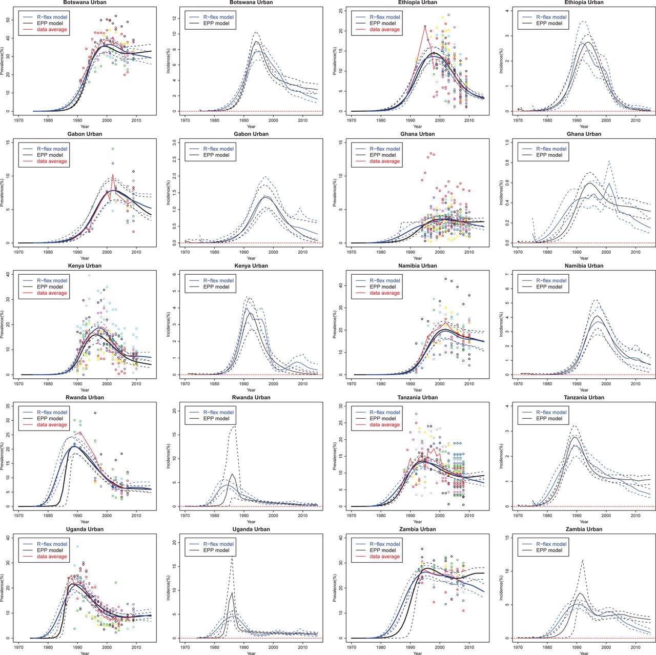
Figure 1 presents the estimation and projection of HIV prevalence and incidence for 10 countries with generalised HIV/AIDS epidemics based on the full prevalence data series. Both classic and flexible models provide reasonable fits to the observed ANC data, and their posterior medians are very close in many cases. The classic EPP model projects HIV incidence in Ethiopia to reach 0% in 2015 with near certainty, which seems overoptimistic. The flexible model implies more uncertainty about HIV incidence in this case. For Rwanda and Uganda, the classic model estimates a sudden increase in prevalence in the early period of the epidemic and the incidence could be as high as 15%; the flexible model estimates a steady increase in prevalence with smoother changes in incidence.

Estimation and projection of HIV prevalence and incidence in 10 countries with generalised epidemics: Botswana, Ethiopia, Gabon, Ghana, Kenya, Namibia, Rwanda, Tanzania, Uganda, and Zambia. Coloured dots show observed prevalence from different sites. The black solid line is the median of the classic Estimation and Projection Package (EPP) model trajectories, the blue solid line is the median of the flexible model trajectories, the dashed lines are the 95% credible intervals, and the red solid line is the data trend averaged over all clinics at each year.
Figure 2 presents flexible model projections from six countries with concentrated HIV/AIDS epidemics. The illustrative examples include the four most common high-risk sub-populations for contracting and transmitting HIV: IDU, MSM, FSW and clients of sex workers (Client). We see that the flexible model works for countries with small amounts of data, such as Moldova MSM and FSW, and for countries with only one site, such as Australia IDU and MSM. However, the prevalence trajectory of the flexible model is mainly driven by the clinic data, for example, Moldova IDU and Nepal IDU. For countries with very sparse data, we may incorporate additional constraints based on expert knowledge to eliminate unrealistic patterns in the flexible model.

Estimation and projection of HIV prevalence among high risk populations in Mexico, Ukraine, Moldova, Nepal, Australia, and Algeria. The high risk populations are sorted by columns: injecting drug users (IDU), men who have sex with men (MSM), female commercial sex workers (FSW), and clients of sex workers (Client). Coloured dots are observed prevalence from different sites. The blue solid line is the median of the flexible model trajectories and the blue dashed lines show the 95% credible intervals of the flexible model trajectories.
Out-of-sample projection
To assess short-term projections, we summarise the coverage and the width of the 95% prediction intervals and MAE for 10 countries with generalised epidemics in table 1. If the model perfectly described the mechanism that generates the data, we would expect 95% of the clinic data to fall between the 2.5th and the 97.5th clinic-specific posterior quantiles. The coverage of the classic EPP model is smaller than 95%, so that the prediction intervals are not wide enough. The flexible model provides improved coverage. For Ethiopia, Ghana and Tanzania, the flexible model provides narrower prediction intervals and better coverage than the classic model. For Gabon, Namibia, Rwanda and Zambia, the flexible model improves coverage by providing wider prediction intervals. When we take the posterior median as the point estimate, the MAE for Ethiopia, Namibia, Tanzania, Uganda and Zambia are substantially reduced by using the flexible model. The flexible model has a larger mean absolute error for Gabon and Botswana but its prediction intervals still cover the data average. Figure 3 shows the out-of-sample projections from the classic EPP model and the flexible model. The data to the right of the vertical line were used only to validate the projection and not for estimating the model parameters.
Comparisons between the classic Estimation and Projection Package (EPP) model and the flexible model: coverage and width of 95% prediction intervals and mean absolute errors of the clinic-specific posterior median for 10 countries with generalised epidemics

Out-of-sample projection of HIV prevalence and incidence in 10 countries with generalised epidemics: Botswana, Ethiopia, Gabon, Ghana, Kenya, Namibia, Rwanda, Tanzania, Uganda, and Zambia. Coloured dots show observed prevalence from different sites. The black solid line is the median of the classic Estimation and Projection Package (EPP) model trajectories sampled from the posterior distribution, the blue solid line is the median of the flexible model trajectories, the dashed lines are the 95% credible intervals, and the red solid line is the data trend averaged over all clinics at each year. The data to the right of the vertical line are used only to validate the projection but not for estimating the model parameters.
We also experimented with other choices of η which is the control parameter for short term projections (see section ‘Additional constraint on projections beyond the last year with data’). Smaller ηs made a stronger equilibrium assumption, and hence did not capture the recent HIV prevalence changes; on the other hand, larger ηs did not provide enough shrinkage towards the equilibrium prevalence, and the prediction intervals were too wide.
Discussion
The flexible epidemiological model implemented in EPP 2011 includes several modifications to the previous approach, namely combining the at-risk and non-at-risk groups, using a stochastic random walk model to allow the infection rate to vary over time, replacing the random starting year of the epidemic t0 with the random seed y(t0) that initialises the epidemic at the fixed starting year, and calibrating the projection towards an equilibrium value for prevalence. The new flexible epidemiological model provides better estimates and short-term projections of HIV/AIDS prevalence in the small number of cases where the classic EPP model has difficulties.
In some settings, users of the flexible model may wish to change the values of a few advanced control parameters. By default, the start year of the epidemic is set at t0=1975 for generalised epidemics and is set from a database of estimated start years for national epidemics. However, the user can define the start year to be any year between 1970 and 1990, and later start years can be used if more appropriate. In our experience, prevalence projections from the flexible model are relatively insensitive to reasonable changes in t0 except in cases where surveillance data only become available near or after the time of peak prevalence. In those cases the early epidemic prevalence trend may vary substantially and should be constrained using prevalence conditions set based on expert knowledge of historical prevalence studies in the country. There are also two variance terms that provide additional control over model output when needed: the variances of the random walk, λ, and the equilibrium parameter, η, which have default values of 0.09. Larger values of λ allow bigger changes in r(t) between years, which can yield more rapid changes in HIV prevalence and incidence and wider CIs. Smaller values of η result in future projections that trend more strongly towards equilibrium for prevalence.
For illustrative purposes, results presented here do not incorporate prevalence data from national population-based surveys. However, in EPP 2011, flexible model estimates and projections are calibrated to these data in the same manner as the classic model.16 The probabilistic framework for the calibration procedure is available in the article by Alkema, Raftery and Clark (2007).17
The random walk model implemented in EPP 2011 is flexible enough to capture a wider variety of epidemic patterns than the classic formulation. However, the algorithm for estimating it converges more slowly than for the classic model, as the flexible model contains a greater number of model parameters to estimate. Model fitting speed tends to be slowest in countries with extensive time series data in large numbers of sites. Additionally, constraints on prevalence in the pre-surveillance period and a constraint on the change of incidence as described in ‘Flexible specification for the infection rate, r(t)’ have sometimes been used to eliminate unrealistic patterns of prevalence and incidence in the flexible model. Those constraints are set based on local expert knowledge, but must be set with caution, because if set too aggressively they may result in a prevalence trajectory that does not match ANC data.
In conclusion, EPP 2011 includes an additional, more flexible modelling option that improves its ability to estimate complicated patterns of HIV prevalence and incidence that have been challenging for the classic model to reproduce. Future improvements to the model should further investigate flexible, parsimonious models that can be estimated efficiently. Such approaches are currently being studied for incorporation into Spectrum/EPP 2013.
Key messages
-
Longer running HIV epidemics are producing more complex patterns of rising and falling incidence, challenging the static model with a fixed infection rate in earlier versions of the United Nations Programme on HIV/AIDS Estimation and Projection Package (EPP).
-
A new ‘Variable-R’ model is proposed in which the infection rate is allowed to vary over time, adjusting as needed to fit the observed prevalence.
-
The model allows fits in countries where the EPP Classic model was not successful: those with rising post-peak prevalence trends or zero incidence due to emptying of the at-risk population.
Acknowledgments
This research was supported by NICHD grant HD054511, a T32 training grant from the National Institute of Allergy and Infectious Diseases (AI 007433) and the Joint United Nations Programme on HIV/AIDS. The authors are grateful to Geoffrey Garnett, Peter Ghys, Karen Stanecki and John Stover for helpful discussions and for sharing data.
References
Footnotes
UNAIDS Report 2012 Guest Editors
Karen Stanecki
Peter D Ghys
Geoff P Garnett
Catherine Mercer
-
Contributions LB, JAS, AER and DRH contributed to conception of the flexible infection-rate model. LB, DRH and TB contributed to model implementation and data analysis. LB, JAS, TB, AER and DRH contributed to writing and editing the manuscript.
-
Funding This research was supported by NICHD grant HD054511, a T32 training grant from the National Institute of Allergy and Infectious Diseases (AI 007433) and the Joint United Nations Programme on HIV/AIDS.
-
Competing interests None.
-
Provenance and peer review Commissioned; externally peer reviewed.
Open Access This is an Open Access article distributed in accordance with the Creative Commons Attribution Non Commercial (CC BY-NC 3.0) license, which permits others to distribute, remix, adapt, build upon this work non-commercially, and license their derivative works on different terms, provided the original work is properly cited and the use is non-commercial. See: http://creativecommons.org/licenses/by-nc/3.0/