Article Text

Abstract
Background Every 2 years, the Joint United Nations Programme on HIV/AIDS (UNAIDS) produces probabilistic estimates and projections of HIV prevalence rates for countries with generalised HIV/AIDS epidemics. To do this they use a simple epidemiological model and data from antenatal clinics and household surveys. The estimates are made using the Bayesian melding method, implemented by the incremental mixture importance sampling technique. This methodology is referred to as the ‘estimation and projection package (EPP) model’. This has worked well for estimating and projecting prevalence in most countries. However, there has recently been an ‘uptick’ in prevalence in Uganda after a long sustained decline, which the EPP model does not predict.
Methods To address this problem, a modification of the EPP model, called the ‘r stochastic model’ is proposed, in which the infection rate is allowed to vary randomly in time and is applied to the entire non-infected population.
Results The resulting method yielded similar estimates of past prevalence to the EPP model for four countries and also similar median (‘best’) projections, but produced prediction intervals whose widths increased over time and that allowed for the possibility of an uptick after a decline. This seems more realistic given the recent Ugandan experience.
- Africa
- antenatal HIV
- epidemiology
- infection
- statistics
This is an open-access article distributed under the terms of the Creative Commons Attribution Non-commercial License, which permits use, distribution, and reproduction in any medium, provided the original work is properly cited, the use is non commercial and is otherwise in compliance with the license. See: http://creativecommons.org/licenses/by-nc/2.0/ and http://creativecommons.org/licenses/by-nc/2.0/legalcode.
Statistics from Altmetric.com
Every 2 years, the Joint United Nations Programme on HIV/AIDS (UNAIDS) publishes updated estimates and projections of the number of people living with HIV/AIDS in the countries with generalised epidemics. Generalised epidemics are defined by the overall prevalence being above 1%, and the epidemic not being confined to particular subgroups; there are approximately 38 such countries.1 The quality of the data available varies widely from country to country. As a result, UNAIDS bases its estimates on a relatively simple method that can be supported by the data in all the countries, and so can give estimates that are comparable between countries. This is based on a simple standard epidemiological model with four adjustable parameters. The data used consist of the proportions of clients of antenatal clinics (ANC) that test positive for HIV in successive years. In some countries these are supplemented by the proportions testing positive for HIV in a nationally representative household survey at one or two time points.
As part of this, statements of uncertainty are also provided. The uncertainty analysis is done using a Bayesian melding method that combines the epidemiological model with a hierarchical random effects model for sampling the variability of the data.2 3 This method was incorporated into the estimation and projection package (EPP) produced by UNAIDS and available for download from http://www.unaids.org. This is used by the UNAIDS Secretariat and also by national officials producing their own estimates and projections. It was used to produce the 2007 update of the UNAIDS estimates and projections.4 5
For most countries, out-of-sample predictive assessments of the type described by Alkema et al2 indicated that the 5-year probabilistic projections produced by the method agreed well with the actual observations. However, the method has had some difficulty in predicting recent data in Uganda, where the epidemic had been declining for a long time. Prevalence increased again in 2006, but the EPP model effectively excludes the possibility of an ‘uptick’ or even a stall in prevalence after a sustained decline.
Here we propose a modification of the EPP model to address this issue. Upticks or stalls in prevalence may be due to changes in the rate of infection, while the infection rate parameter in the EPP model, r, is assumed to be constant over time. We modified the model by allowing the infection rate parameter to vary stochastically over time; we refer to this as the r stochastic model. We applied the new model to the data from Uganda, and show that when used to generate predictions for the period 2003–7 based on data up to 2002, it does allow for the possibility of an uptick in prevalence after 2002, unlike the EPP model.
The article is organised as follows. In the Methods section we review the EPP model, describe the new r stochastic model, and outline the Bayesian estimation method we use. In the Results section, we give the results for Uganda, and also for Kenya, Rwanda and Gabon.
Methods
The estimation and projection package
The EPP model uses a simple susceptible–infected–removed epidemiological model that incorporates population change over time by fitting the four adjustable input parameters r, t0, f0, and ϕ, where r is the rate of infection, t0 is the start year of the epidemic, f0 is the initial fraction of the adult population at risk of infection, and ϕ is a behaviour change parameter. The output ρ is a sequence of yearly HIV prevalence rates.
The EPP model divides the population at time t into three groups: a not-at-risk group, X(t), an at-risk group, Z(t) and an infected group, Y(t). The model assumes a constant non-AIDS mortality rate μ and a constant fertility rate, and does not represent migration or age structure. The rates at which the sizes of the groups change are described by three differential equations:
Survival after infection is assumed to have a Weibull (2.4, 12.8) distribution, which implies that the median survival time is 11 years.6 In the start year t0 of the epidemic, a fraction λ(t0)=0.1% of the at-risk group Z moves to the infected group Y. The population being modelled is aged over 15 years. The number of new members at time t, E(t), depends on the population size 15 years ago, the birth rate and the survival rate from birth to age 15 years. When individuals survive to age 15 years, they are assigned to either the not-at-risk group, X(t), or the at-risk group, Z(t). The fraction of the new 15-year-old members entering the at-risk group, Z(t), is
The Bayesian melding approach7 was applied to the EPP model by Alkema et al.2 It proceeds as follows. A prior distribution is specified for θ=(r, t0, f0, ϕ). The UNAIDS reference group on estimates, modelling and projections agreed on a default prior distribution, but users can specify their own. The observed ANC and national population-based survey data give the likelihood L(ρ) for the model output, using a hierarchical random effects model. A prior on the model output ρ can also be specified; in the current software this is restricted to being uniform between specified bounds for specific years.
In the 2007 version of the EPP software, the Bayesian melding procedure computed the posterior distributions using the sampling–importance–resampling algorithm of Rubin,8 9 with the prior distribution as importance sampling distribution. Raftery and Bao10 proposed a more efficient sampling strategy called incremental mixture importance sampling (IMIS), which was implemented in the 2009 version of the EPP software.11 It is generic, relatively simple to implement and explain, and works well for countries for which the sampling–importance–resampling algorithm is inefficient.
The r stochastic model
The EPP model has worked well for estimating and projecting HIV prevalence in most countries. However, prevalence in Uganda has recently gone back up after a long decline, and the EPP model cannot represent this. Also, its probabilistic projections for other countries that have had a sustained decline essentially exclude the possibility of an uptick or even a stall, which seems unrealistic given the recent experience in Uganda.
To allow the EPP model to represent an uptick in prevalence after a sustained decline, as was observed in Uganda, we propose a modification called the r stochastic model, which allows the rate of infection to vary in time. It also drops the distinction between individuals at risk and those not at risk of infection, treating all HIV-negative persons as being at risk. It thus divides the population at time t into two groups rather than three: a non-infected group, Z(t), and an infected group, Y(t). The rates at which the sizes of the groups change are described by two differential equations:
The infection rate, r(t), is the average number of persons infected by one HIV-positive person in year t. We model r(t) as a random walk on the log scale, as follows. We model the first differences of the log r(t) process as independent and identically distributed normal random variables with mean zero and SD σ: ∆(t)=log r(t)−log r(t−1)∼N(0, σ2). All the other parameters are defined in the same way as in the standard EPP model. The incidence is defined as
Estimation
We carry out Bayesian estimation of the input parameters t0, σ2 and r(t) with the following prior distributions:
We chose ν0=20 and β=0.005, so that the prior SD, σ, has median 0.072, 2.5th percentile 0.054 and 97.5th percentile 0.102. This is wide enough to accommodate the observed changes in all the countries we have considered. To implement the Bayesian estimation, we use the IMIS algorithm of Raftery and Bao.10
To apply IMIS to the r stochastic model, we need to modify it. This is because IMIS is designed for continuous parameters, and the start year t0 of the epidemic is a discrete parameter, as it can take only integer values. To deal with this, for each value of t0 (1970, 1971… 1990), we created a sample from the posterior distribution of the other parameters using IMIS, which can be done because the other parameters are continuous. For each fixed t0, we chose N0=10 000 initial samples, B=1000 new samples at each iteration, and J=1000 resampled values.
To improve sampling efficiency, we used the IMIS-opt version of the IMIS algorithm with a single optimiser inserted after the initial stage. We further improved efficiency by integrating out σ2 analytically, so that it is not included in the sampling algorithm. When this is done, the joint prior distribution of the ∆(t) values is a multivariate t distribution with ν0 degrees of freedom, mean vector 0, and matrix parameter βI.
The posterior samples under different t0 values are then combined as follows. For each t0 a subsample of the posterior sample is drawn, with a sample size proportional to the posterior probability of t0. This is in turn proportional to the integrated likelihood
Results
HIV prevalence estimation and projection based on ANC data
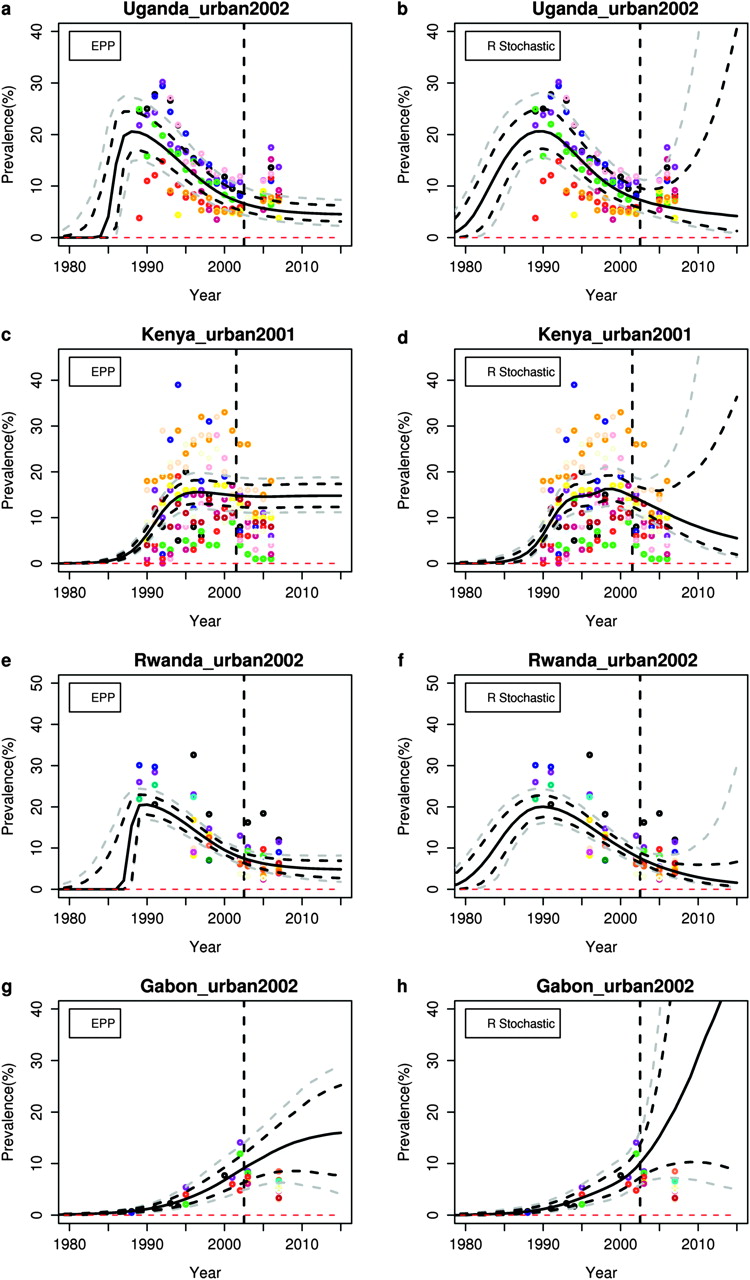
UNAIDS provides 5-year projections of prevalence, and figure 1 shows the estimates and projections from the EPP model and the r stochastic model up to 2015 for illustrative data for the urban areas of Uganda, Kenya, Rwanda and Gabon. These countries are at different stages of the epidemic and have very different amounts of data. Note that the results are based on illustrative HIV prevalence data from ANC in these countries, which may not be complete or accurate. These results should therefore also not be seen as replacing or competing with official estimates as regularly published by countries and UNAIDS. This is HIV prevalence data from ANC but for all urban areas.

Estimation and projection: (A) Uganda estimation and projection package (EPP) prevalence; (B) Uganda r stochastic prevalence; (C) Kenya EPP prevalence; (D) Kenya r stochastic prevalence; (E) Rwanda EPP prevalence; (F) Rwanda r stochastic prevalence; (G) Gabon EPP prevalence; (H) Gabon r stochastic prevalence. The black solid line is the posterior median, the grey and black dashed lines show the 95% and 80% posterior intervals, respectively.
For Uganda, ANC data on HIV prevalence were first collected in 1989. Prevalence peaked around that time and then declined steadily through the 1990s, and then stabilised before increasing again in 2006. The EPP model cannot capture the uptick in 2006, but the r stochastic model does allow for this possibility.
In Kenya, prevalence peaked in the mid-1990s, and since then has been declining. The EPP model projects that the epidemic will disappear by 2015 with near certainty, which seems overly optimistic, particularly in light of the Ugandan experience. The r stochastic model gives similar estimates to the EPP model, but its probabilistic projection allows for the possibility of stabilisation or even an uptick by 2015, which seems more realistic.
For Rwanda, the probabilistic projection from the EPP model implies that there will be neither a further decline nor an increase before 2015. The r stochastic model gives similar estimates to the EPP model for 1990–2007, but its probabilistic projection interval is wider and increases with time, allowing for either a continued modest decline or an uptick.
Gabon is an example of a country with few ANC data, but where the EPP model works well nevertheless. The r stochastic model gives similar results to the EPP model, with a slightly wider prediction interval for 2015. This reflects the fact that it allows for the possibility of an uptick, unlike the EPP model. This indicates that the r stochastic model can work well in spite of the fact that it makes fewer assumptions than the EPP model, even when prevalence data are sparse.
Out-of-sample projection results
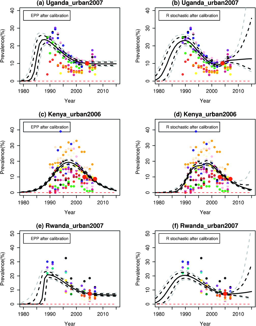
To assess the predictions of the EPP and r stochastic models, we removed the last 5 years of data, re-estimated the models, and compared their projections with what was subsequently observed. We did this for Uganda, Kenya, Rwanda and Gabon. The results are shown in figure 2.
Out-of-sample projection: (A) Uganda estimation and projection package (EPP) prevalence; (B) Uganda r stochastic prevalence; (C) Kenya EPP prevalence; (D) Kenya r stochastic prevalence; (E) Rwanda EPP prevalence; (F) Rwanda r stochastic prevalence; (E) Gabon EPP prevalence; (F) Gabon r stochastic prevalence. The data to the right of the vertical line are used only to validate the projection but not for estimating the model parameters. The black solid line is the posterior median, the grey and black dashed lines show the 95% and 80% posterior intervals, respectively.
For Uganda, the probabilistic projection intervals from the EPP model clearly missed the increase in prevalence in 2006. The posterior median projection from the r stochastic model did decline after 2002, as for the EPP model, but it produced prediction intervals whose widths increased over time and that did encompass the observed prevalence increase.
For Kenya, the EPP model projected a flat trend and excluded a substantial decline by 2007, although a decline did occur (see figure 1). The r stochastic model projected a decline of the kind that actually occurred (compare figure 2(D) with figures 1C, D). More importantly, the r stochastic model captured the uncertainty in the projection more fully, allowing for the possibility of either a decline (which did happen) or an uptick (which did not happen in Kenya but did in Uganda).
For Rwanda, the out-of-sample projections from the two models are similar, although the intervals from the r stochastic model are wider. Both capture the subsequent outcomes fairly well.
For Gabon, the out-of-sample projection is based on very few data points up to 2002. Both the EPP model and the r stochastic model missed projecting the downturn in prevalence from 2003 to 2007. The projections for Gabon from 2007 based on all the available data are similar for EPP and the r stochastic model, and both seem reasonable. This suggests that caution should be exercised in making projections based on very sparse past data.
Results calibrated to national population-based surveys
The results we have shown so far are based only on the ANC data, which tend to be biased upwards. Several of the countries with generalised HIV/AIDS epidemics have also had nationally representative household-based demographic and health surveys that have included HIV tests and so provide roughly unbiased estimates of HIV prevalence.
Alkema et al3 have developed a method for probabilistic estimation and projection of the epidemic that takes account of both the national population-based survey and the ANC data; this is now incorporated in the EPP software. Essentially, trends are based on the ANC data, but estimates are adjusted to match the national population-based survey results, taken to be unbiased. The national population-based survey estimates are also more precise than the ANC estimates, ie, they tend to have a lower variance, and so incorporating the national population-based survey data reduces both bias and uncertainty.
Calibrated estimates and projections of prevalence from the EPP and r stochastic models for the three countries with national population-based surveys are shown in figure 3.
Results from the estimation and projection package (EPP) and r stochastic models calibrated by population-based surveys: (A) Uganda EPP prevalence; (B) Uganda r stochastic prevalence; (C) Kenya EPP prevalence; (D) Kenya r stochastic prevalence; (E) Rwanda EPP prevalence; (F) Rwanda r stochastic prevalence. The red dots are estimated from the population-based surveys. The black solid line is the posterior median, the grey and black dashed lines show the 95% and 80% posterior intervals, respectively.
Estimating incidence
Incidence at time t, I(t), can be estimated from the calibrated prevalence estimates using the following equations:
The estimated incidence for the three countries with national population-based surveys from both models is shown in figure 4. For all three countries, the projection intervals for future incidence from the r stochastic model are much wider than those from the EPP model.

Estimates of HIV incidence from the estimation and projection package (EPP) and r stochastic models calibrated by population-based surveys: (A) Uganda EPP incidence; (B) Uganda r stochastic incidence; (C) Kenya EPP incidence; (D) Kenya r stochastic incidence; (E) Rwanda EPP incidence; (F) Rwanda r stochastic incidence. The vertical line indicates the end year of observed antenatal clinic data. The black solid line is the posterior median, the grey and black dashed lines show the 95% and 80% posterior intervals, respectively.
Discussion
The current EPP model has had some difficulty in projecting HIV prevalence in countries that have had a substantial decline. In particular, in Uganda prevalence has gone up again after a long decline, and the EPP model cannot represent this. For other countries that have had declines, EPP projects a continuing decline, with essentially no probability assigned to an uptick, which seems unrealistic in light of Uganda's experience. To address this issue, EPP 2009 has the ϕ-shift feature, which handles upticks in prevalence, but for which the theoretical framework is not well developed and for which the performance with different datasets has not been rigorously investigated.11
In this article, we have proposed the r stochastic model in which the rate of infection is allowed to vary randomly over time, and is applied to the entire non-infected population; the separate at-risk category in the EPP model is removed. For estimation of past prevalence this gives similar results to EPP, and it also gives similar median (‘best’) projections. However, it yields prediction intervals whose widths increase with time into the future, and that allow for the possibility of upticks in prevalence after a decline. This seems realistic, especially in view of the recent experience of Uganda. It also allows the incorporation of national population-based surveys, similarly to the EPP model.
To estimate the model we have used Bayesian melding implemented with the IMIS method. IMIS has been applied with success to the four-parameter EPP model and also to Heuveline's age-specific demographic model for HIV/AIDS, which has approximately 30 parameters.12 In our experience, the computing time needed to estimate the r stochastic model with a fixed t0 is similar to that needed to run the EPP model.
As implemented in this article, the method takes no specific account of future antiretroviral therapy use. The EPP model does allow one to take account of future antiretroviral therapy use, using assumptions specified by the user. This could be incorporated in the r stochastic model in a similar way.
Acknowledgments
The authors are grateful to Tim Brown, Dan Hogan, Peter Ghys, John Stover and Joshua Salomon for helpful discussions and for sharing data, and to the Editor and two referees for helpful comments.
Footnotes
Funding This research was supported by NICHD grant HD054511.
Competing interests None.
Provenance and peer review Not commissioned; externally peer reviewed.